Probability density functions (PDFs)
A probability density function (PDF) is a function that represents the likelihood of an outcome of a probability "experiment." PDFs generally model continuous random variables, rather than discrete variables, though they can be applied to both.
The PDF gives the probability that the value of a continuous random variable will fall within some range of that variable. It can't predict absolute likelihood because that isn't well-defined for a continuous random variable. "Continuous" means having an infinite range of values, therefore the probability of any one specific outcome among them is zero.
One of the most recognizable PDFs is the Normal or Gaussian distribution function (named for Carl Friedrich Gauss). It's also known as the "bell curve." It looks like this:
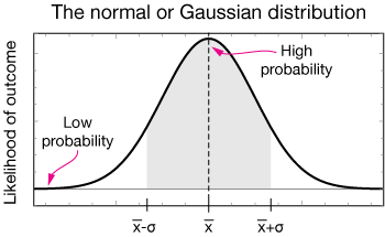
The Gaussian curve shows that the most-likely value is the mean, $\bar{x}$. We also define two points, $\bar{x} ± \sigma$, where $\sigma$ is the standard deviation and $\sigma^2$ is called the "variance of the distribution."
As an example of how such a distribution is used, Let's take a look at the distribution of heights of adult women living in the U.S. in 2016. The horizontal axis is height, from shorter on the left to taller on the right. The height of the curve is proportional to the number of women with height x. The average height, $\bar{x}$, was 65.5 inches.
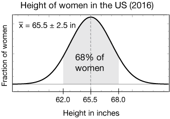
The probability of a height falling within some range of heights is given by the area under the curve between those two heights. For the Gaussian distribution, there is a specific range, $\bar{x} ± \sigma$ , which encloses 68% of the total probability. It shows that 68% of all U.S. women in 2016 had heights between 65.5 - 2.5 = 63 inches and 65.5 + 2.5 = 68 inches. In obtaining a curve like this, we tweak a small set of parameters (just $\bar x$ and $\sigma$ in this case) to fit a Gaussian curve to the data.
In this section we'll take a closer look at the Gaussian or "normal" probability distrbution, its uses and properties. The normal distribution is the most commonly-used probability distribution function.
Pro tip
In this section, like out in the world, the terms Normal distribution and Guassian distribution will be used interchangeably. Get used to hearing and reading both, but feel free to choose your favorite. "Gaussian" is capitalized because Gauss is a person's name.
Why use the Gaussian distribution?
It's very common
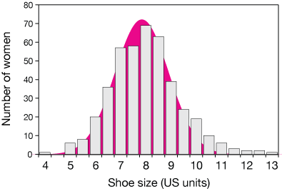
Distributions of many variable or random error in measurements are very nearly Normal – by which we mean distributed according to the Gaussian or normal distribution function. Measurements of lengths or heights, test scores or IQ scores, and shoe size are just a few examples. Here are bar-chart representations of a couple of these
Shoe size (US) for 424 women
Weight of top 50 NFL offensive tackles
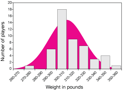
In the second example, I intentionally chose a data set that was small – just 50 samples. Although I'm reasonably confident that, given many more samples, the histogram (bar chart) would look more and more like a normal curve, it might be a stretch to suggest that from this small set of data points. There's a little more about small and large data sets below.
Mathematical ease
Relatively speaking, the normal distribution function is fairly easy to work with. Some aspects (like integrating the function) might be difficult to learn, but they're still well-understood. Many of the statistical tools we use to analyze the quality of a data set are derived from an underlying assumption of a normal distribution.
Central limit theorem
There's another section dedicated to the central limit theorem, but here is one example.
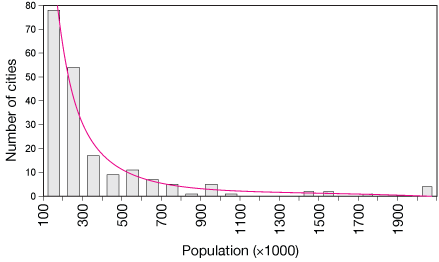
Number of US cities in population ranges (in thousands of people) in 2019
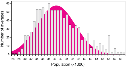
Distribution of 1000 averages of 100 randomly-selected US city populations
The upper graph shows the number of US cities (in 2019) grouped by population. Clearly there are many more cities of population around 100,000 people than much larger cities. This is not a Gaussian distribution at all. It's more like a decaying exponential graph.
However, when we take random samples of these cities, and calculate averages of their populations, the resulting distribution of averages will become more and more like a normal distribution as we increase the number of averages. In the lower graph, samples of 100 cities were drawn from a pool of 200 (the sample size of the upper graph), and averaged. That was done 1000 times, and the results were binned and plotted. The result is very nearly normal, but still just a little skewed to the left, like the parent distribution..
This is another underlying reason for using the normal distribution: random sampling of almost any distribution, provided we take enough samples, and provided that the results are due to a variety of unrelated (uncorrelated) inputs, tends to produce a distribution of averages that is nearly normal.
Mathematical form
Mathematically, the Gaussian or normal distribution has the form
$$F(x) = \frac{1}{\sigma \sqrt{2\pi}} exp\left( \frac{-(x - \bar{x})^2}{2 \sigma^2} \right),$$
where
- The exp function is just the normal exponential function, $e^a,$ but it's written this way when the exponent would be cumbersome written as a superscript.
- $F$ stands for frequency – the likelihood of obtaining a given result,
- $\sigma$ (Greek sigma) is the standard deviation, a common measure of the width of the distribution function (more on that later),
- $x$ is the continuous independent variable,
- and $\bar{x}$ is the mean value, the x (domain) location of the peak of the distribution in this case. In some circumstances, $\bar x$ is written as $\mu$.
The factor $1/\sigma \sqrt{2\pi}$ is a normalization factor. It ensures that for any value of σ or $\bar{x},$, the total area under the curve, which represents the probability that some outcome will occur, is 1.
The plot on the right shows the Gaussian distribution for a probability experiment with a $\bar{x} = 50,$ and $\sigma = 5.$ By moving the slider, you can change σ between 5 and 50.
Notice that as you change σ, the peak of the distribution decreases, but the rest of the function broadens to keep the total area under the curve constant. When σ is small relative to the mean, the distribution might represent a set of measurements with high precision (low random error). When it's large, there is more uncertainty about the location of the true mean.
Mathematical (calculus) digression: What is σ?
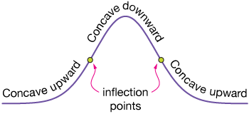
The standard deviation, σ, is the distance from the mean of our distribution to a set of unique points, inflection points, where the curvature of the graph changes from concave-upward to concave-downward, or the reverse. You may know that inflection points are found by setting the second derivative of a function equal to zero and solving for x. Let's do that for the Gaussian distribution. We'll let $\bar{x} = 0,$ which simplifies the function a bit and just centers it at x = 0.
$$ \begin{align} F'(x) &= \frac{1}{\sigma \sqrt{2\pi}} e^{\frac{-x^2}{2\sigma^2}} \left( \frac{-2x}{2 \sigma^2} \right) \\[5pt] &= \frac{1}{\sigma^3 \sqrt{2 \pi}} x e^{\frac{-x^2}{2\sigma^2}} \end{align}$$
Now the second derivative is
$$ \begin{align} F''(x) &= \frac{1}{\sigma^3\sqrt{2\pi}} \left( e^{\frac{-x^2}{2\sigma^2}} + x e^{\frac{-x^2}{2\sigma^2}} \left( \frac{-2x}{2\sigma^2} \right) \right) \\[5pt] &= \frac{1}{\sigma^3\sqrt{2\pi}} \left( e^{\frac{-x^2}{2\sigma^2}} \left( 1 - \frac{x^2}{\sigma^2} \right) \right) \end{align}$$
Now set that expression equal to zero to find the inflection points. Notice that the constant term on the right will just divide away into the zero, giving
$$e^{\frac{-x^2}{2\sigma^2}} \left( 1 - \frac{x^2}{ \sigma^2} \right) = 0$$
Now the exponential term is never zero, so the only condition that makes this equation true is if
$$x^2 = \sigma^2,$$
or
$$x = \sigma$$
So σ (actually $\bar{x} ± \sigma$) does indeed give the location of the inflection points.
This unique set of points on our curve ensures that we're always referencing the same width from distribution to distribution.
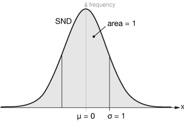
The Standard Normal Distribution (SND)
A very important version of the Gaussian or Normal distribution is the Standard Normal Distribution (SND). It is simply a Gaussian distribution with a mean of zero $(\mu = 0)$ and a standard deviation of 1 $(\sigma = 1)$. Any Normal distribution can be scaled into the SND by dividing by the mean and standard deviation of the original distribution.
The functional form of the SND is
$$F(x) = \frac{1}{\sqrt{2 \pi}} e^{\frac{-x^2}{2}}$$
Area under the SND
The total area under the SND is one. In the functional form, the factor $1/\sqrt{2 \pi}$, the normalization constant, ensures that. The derivation of that constant is illustrated in the box below. It involves a bit of integral calculus in two dimensions, so skip it if you can't follow it yet.
We can add up areas under the SND very easily, either using technology – computer programs, calculators &c., or tables, which are compiled in most statistical textbooks.
Combined with the Z-score (see below), we can use the SND to determine probabilities that events will or will not occur.
Finding the area under the curve: The Gaussian integral
What we need to do to establish the formula for the SND so that the area under the curve equals one, that is to say, the function is normalized, is to solve the integral equation:
$$\int_{-\infty}^{\infty} e^{-\frac{x^2}{2}} dx = 1 \tag{1}$$
Well, that's a tricky integral. It would be nice if there was an extra $x$ in there, so that the integrand was something like $e^{-x^2/2} \color{red}{x} \, dx$, but there is not. There is a trick, though, and that's to do it as a two-dimensional integral and convert to polar coordinates. Here it is: First, let's let
$$\int_{-\infty}^{\infty} e^{-\frac{x^2}{2}} dx = I$$
Then we can change the integral to a two-dimensional one:
$$ \begin{align} \int_{-\infty}^{\infty} &\int_{-\infty}^{\infty} e^{-\frac{x^2}{2}} e^{-\frac{y^2}{2}} dx dy \\[5pt] &= \int_{-\infty}^{\infty} e^{-\frac{y^2}{2}} \int_{-\infty}^{\infty} e^{-\frac{x^2}{2}} dx dy \\[5pt] &= I \int_{-\infty}^{\infty} e^{-\frac{y^2}{2}} dy \\[5pt] &= I^2 \end{align}$$
So, with the integrand written slightly differently, we have
$$\int_{-\infty}^{\infty} \int_{-\infty}^{\infty} e^{-\bigg( \frac{x^2 + y^2}{2} \bigg)} dx dy = I^2$$
Now we can convert to polar coordinates. Recall that
$$ \begin{align} r^2 &= x^2 + y^2 \; \text{and} \\[5pt] dx dy \; &\rightarrow \; r \, dr d\theta \end{align}$$
where the integral over r goes from 0 to ∞ and the integral over θ goes from 0 to 2π. The new integral is
$$\int_0^{\infty} \int_0^{2 \pi} e^{\frac{-r^2}{2}} r \, dr \, d\theta$$
Now that integral can be done using simple substitution. Let
$$u = \frac{r^2}{2} \; \rightarrow \; du = -r \, dr$$
The new integral is
$$\int_0^{\infty} \int_0^{2 \pi} e^{-u} du \, d\theta$$
The integral over θ reduces to
$$\theta \, \bigg|_0^{2 \pi} = 2 \pi$$
and the integral over r is
$$\frac{-1}{e^u} \, \bigg|_0^{\infty} = 0 - (-1) = 1$$
So finally we have $I^2 = 2 \pi$, which gives us $I = \sqrt{2 \pi}$.
Finishing off our normalization from equation (1) gives us the normalization constant,
$$I = 1 \; \rightarrow \; I = \frac{1}{\sqrt{2 \pi}}$$
Our normalized Standard Normal Distribution function is
$$F(x) = \frac{1}{\sqrt{2 \pi}} e^{- \frac{x^2}{2}}$$
The Z-score
The Z-score is a way of locating a point in the domain of a Normal distribution. The location is specified by the number of standard deviations $(\sigma)$ to the right or left of the mean, so Z-scores are a way of comparing locations in different distributions. The Z-score for a location $x$ in the domain of a Gaussian distribution is
$$Z = \frac{x - \bar x}{\sigma}$$
Here's an example of how the Z-score is used. Let's say that we have a Gaussian or Normal distribution with a mean of 65 and a standard deviation of $\sigma = 4$: $\bar x = 65 ± 4$. We'd like to know, for example, what the probability of obtaining a result of 68 or higher. First we calculate the Z-score for $x = 68$:
$$ \begin{align} Z &= \frac{x - \bar x}{\sigma} \\[5pt] &= \frac{68 - 65}{4} = \frac{3}{4} = 0.75 \end{align}$$
Here's what that looks like graphically:
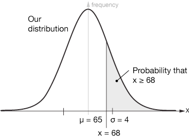
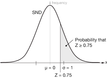
If we translate that Z-score to the SND, it looks the same, but now we can calculate the probabilities on either side. If we want the probability of obtaining a result greater than or equal to 68 we just need to calculate the area of the gray region. That can be done in two main ways, by using tables printed at the back of most statistics textbooks or available on-line, or using technology, such as a TI-84 calculator.
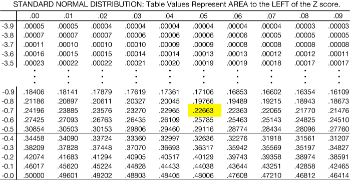
The table below is a partial example of a Standard Normal Table of Areas. Many of the rows are left out for brevity. It's important to get a feel for the table you're using. This one lists negative values on the Z-score; that's to the left of the mean. Some are a bit different. Not to worry, though, because the SND is left-right symmetric. It also lists areas integrated (added up) from the left. Looking at the table we read down the first column until we get to the first digit of our Z-score, 0.7 (ignoring the negative sign), then over across the columns until we get to the column labeled 0.05. At the intersection, we read the area from the extreme left of the distribution to the Z = -0.75 mark, 0.22663. That means that there is a 22.6% chance of obtaining an x-value of 68 or higher from this distribution.
Using a calculator to find probability
On the TI-84 calculator there is a handy program for calculating areas from Z-scores. Older models only integrate those areas from the left, but newer ones can work from both sides. To access the program, hit [2ND] [
Here's the screen you'll see after hitting [2ND] [

In this version of the program we can enter both limits. We'll place the Z-score, $Z = 0.75$ as the left limit. Then we want to integrate under the function far out into the wings. It's customary to put a very large number here, usually $1 \times 10^{99}$. Actually even a number like 1000 is usually fine. You choose, but test your method against an outer limit of $1 \times 10^{99}$.
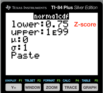
The mean $(\mu)$ and standard deviation $(\sigma)$ are zero and one for the SND. Here's the output. You can see that the area is the same as we got using the table.
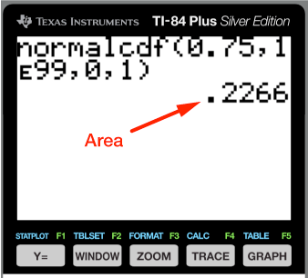
The normalcdf function can also be used directly on the original distribution, by entering the mean and standard deviation of that distribution. Try it; the area will be the same.
Practice problems
-
For a distribution with $\mu = 2.343$ and $\sigma = 0.293$, determine the probability of obtaining a result less than 2.00.
Solution
The Z-score is
$$Z = \frac{2.00 - 2.345}{0.293} = -1.1774$$
The area, using a calculator, is
normalcdf(-1E99, -1.17744, 0, 1) = 0.1195
So the probability of obtaining a result of less than 2.00 from this distribution is just about 12%.
-
For a distribution with $\mu = 24.0$ and a standard deviation of $\sigma = 3.5$, calculate the probability of obtaining a result between 21.0 and 22.0
Solution
The Z-scores for the endpoints are:
$$ \begin{align} Z_1 &= \frac{21.0 - 24.0}{3.5} = -0.8571 \\[5pt] Z_2 &= \frac{22.0 - 24.0}{3.5} = -0.5714 \end{align}$$
We can find the probability directly on a calculator like this:
normalcdf(-0.8571, -0.5714, 0, 1) = 0.0882
The probability of obtaining a result between 21 and 22 is just under 9%.
-
Of 24 basketball games played by the Spartans in 1980, the total points scored by the team were
54 84 89 73 62 69 59 41 48 48 64 80 43 58 67 70 80 74 78 62 68 77 87 90 Determine the probability that the Spartans would score between 70 and 80 points during that season.
Solution
Using a list of the scores on a TI-84 calculator, and calculating the 1-variable statistics gives $\mu = 67.71 ± 14.3$, where the ± value is one standard deviation $(\sigma)$. Then the Z-scores for point totals of 79 and 80 are
$$ \begin{align} Z_1 &= \frac{70 - 68}{14} = 0.1429 \\[5pt] Z_2 &= \frac{80 - 68}{14} = 0.8571 \end{align}$$
We can find the probability directly on a calculator like this:
normalcdf(0.1429, 0.8571, 0, 1) = 0.2475
The probability that the Spartans scored between 70 and 80 points was about 25%.
-
The mean of a distribution is $\mu = 274$. If there is an 18.5% chance of measuring a value of $x$ that is 292 or higher, calculate the standard deviation of the distribution of $x$. (Hint: The invNorm function of the TI-84 calculator will give you the Z-score for a given area).
Solution
The invNorm function is found by hitting [2ND][
DISTR ] and selecting the 3rd option. If we plug in an area of 0.185 like this:invNorm(0.185, 0, 1) = -0.8965
That result is an artifact of the TI-84 program. It integrates or adds up area from the left to the right, so it's giving us the Z-score that would block out 18.5% of the probability on the left side of the Normal distribution. We're lookijg for the area on the right. That's OK because the distribution is symmetric. The Z-score we're looking for is $Z = + 0.8965$.
Now we can rearrange the Z-score formula to find $\sigma$:
$$ \begin{align} Z &= \frac{x - \mu}{\sigma} \\[5pt] \sigma &= \frac{x - \mu}{Z} \\[5pt] \sigma &= \frac{292 - 274}{0.8965} = 20.08 \end{align}$$
-
The Wechsler Adult Intelligence Test comprises some smaller subtests. On one subtest, the raw scores have a mean of 45 and a standard deviation of 7. Assuming that the raw scores are distributed normally, what score represents the 70th percentile? That is, what number separates the lower 70% of the distribution?
Solution
The Z-score for an area under the SND of 0.7 is given by
invNorm(0.7, 0, 1) = 0.5244
That's just a little over half a standard deviation greater than the mean. That would give us a score of
$$x = 45 + 0.5244(7) = 48.67$$
We'll round that to 49. A score of 49 means that the test taker scored higher than 70% of the people who took the test – and lower than 30%.
-
Let's say that the mean of an SAT test in a particular year was $\mu = 500$ with a standard deviation of $\sigma = 100$. What would be the minimum score a taker would have to make in order to be in the top 15% (that is, the 85th percentile) of the distribution, assuming it's a Normal distribution.
Solution
To block out 85% of the SND, the Z-score would have to be
invNorm(0.85, 0, 1) = 1.0364
So the score would be
$$x = 500 + 1.0364(100) = 603.64$$
We'll round that to 604. In order to be in the 85th percentile, a test taker would have to score a 604
The 68-95-99.7 rule
It's convenient to know the area of a Normal distribution enclosed by the mean plus and minus multiples of the standard deviation. That is, we'd like to know how much area is enclosed by
- $\mu ± \sigma$,
- $\mu ± 2\sigma$ and
- $\mu ± 3\sigma$
Those areas are about 68%, 95% and 99.7%, respectively. Those are illustrated in the figure below, and the table lists areas enclosed by a few multiples of $\sigma$.

Fractions of the area under the Gaussian curve (in percent) enclosed by multiples (n) of σ*
| $n$ | % prob | $n$ | % prob |
|---|---|---|---|
| 0.0 | 0.0 | 1.4 | 83.8 |
| 0.2 | 15.8 | 1.6 | 89.0 |
| 0.4 | 31.0 | 1.8 | 92.8 |
| 0.6 | 45.2 | 2.0 | 95.4 |
| 0.8 | 28.8 | 2.2 | 97.2 |
| 1.0 | 34.1 | 2.4 | 98.4 |
| 1.2 | 77.0 | 2.8 | 99.4 |
*
The Greek alphabet
| alpha | Α | α |
| beta | Β | β |
| gamma | Γ | γ |
| delta | Δ | δ |
| epsilon | Ε | ε |
| zeta | Ζ | ζ |
| eta | Η | η |
| theta | Θ | θ |
| iota | Ι | ι |
| kappa | Κ | κ |
| lambda | Λ | λ |
| mu | Μ | μ |
| nu | Ν | ν |
| xi | Ξ | ξ |
| omicron | Ο | ο |
| pi | Π | π |
| rho | Ρ | ρ |
| sigma | Σ | σ |
| tau | Τ | τ |
| upsilon | Υ | υ |
| phi | Φ | φ |
| chi | Χ | χ |
| psi | Ψ | ψ |
| omega | Ω | ω |
discrete
Discrete means individually separate and distinct. In mathematics, a discrete varable might only take on integer values, or values from a set {a, b, c, ... d}. In quantum mechanics, things the size of atoms and molecules can have only discrete energies, E1 or E2, but nothing in between, for example.
artifact
In math and science, an artifact is something that happens as the result of applying a certain method to a problem. It is usually expected and easily corrected for if needed. For example, in some X-ray scans, parts of the image might look like a tumor, but qualified interpreters might recognize the object as having resulted from some well-known phenomenon having to do with the imaging technique.

![]()
xaktly.com by Dr. Jeff Cruzan is licensed under a Creative Commons Attribution-NonCommercial-ShareAlike 3.0 Unported License. © 2016-2025, Jeff Cruzan. All text and images on this website not specifically attributed to another source were created by me and I reserve all rights as to their use. Any opinions expressed on this website are entirely mine, and do not necessarily reflect the views of any of my employers. Please feel free to send any questions or comments to jeff.cruzan@verizon.net.