Binomial situations
Many of the situations in which we want to make a statistical analysis take the form of a dichotomy: Something is either true or it is not. An object is either blue or it is red. A person either approves of a political leader or she does not, and so on.
In the language of binomial distributions, we often cast these in terms of failures or successes.
The binomial "setting"
To be able to take advantage of some of the rules we'll develop for binomial situations, we'll have to carefully define when we can use them – when we're in a bionomial setting. Four conditions must be met:
- The situation is binary. That is, each outcome can be classified in some sense as either a "sucesses" or a "failure."
- Each trial or experiment must be independent of all others. Knowing the result of one trial must have no effect on the others. This will become a little tricky when we start choosing samples of populations without replacement, but we'll get to that as we need to; .
- The number of trials $(n)$ in each experiment or random process must be the same. If we're drawing ten samples from a population and examining them for success or failure, then we need to keep using a sample size of ten; $n$ is constant
- The probability of success, which we'll call $p$, must be the same for each trial.
Binomial situation: BINS
You can remember the requirements for using a binomial distribution using the acronym BINS.
- Binary – is this a "success" vs. "failure" situation?
- Independent – Are the trials independent?
- Number – is the number of trials constant?
- Success? – is success clearly defined with a fixed probability, $p$ ?
Note: The binomial distribution is a discrete probability distribution, not a continuous one.
Binomial probabilities by example
Let's imagine doing a taste test to see who likes which diet soda better, Coke™ or Pepsi™.

For simplicity, let's choose samples of three people to ask a binary question: Is Diet Coke™ your favorite (of the two) or not? We'll assume here (and it may not be the case) that the probability is $p = 0.5$. Now at first blush, there are four different outcomes for three selections. They are:
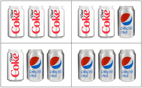
That is, either all three people like Coke, two of three do, 1 of three do, or none does.
Now let's add up all of the probabilities. We have P(C) = 0.5 and P(P) = 0.5 for the probabilities of choosing a Coke or Pepsi. So here are our probabilities:
$$ \begin{align} P(CCC) &= 0.5^3 = 0.125 \\[5pt] P(CPP) &= 0.5^2(1-0.5) = 0.125 \\[5pt] P(CCP) &= 0.5(1-0.5)^2 = 0.125 \\[5pt] P(PPP) &= (1-0.5)^2 = 0.125 \end{align}$$
Now the sum of these probabilities is 0.5, so that doesn't feel too good. We've exhasted the possibilities that something will happen, but our probabilities don't sum to one, so we've obviously missed something.
Here's what we missed:

Notice that for the combinations containing one Coke and two Pepsis or two Cokes and one Pepsi, there are three ways that those combinations could have occurred:
$$ \begin{align} CCP \phantom{000} CPC \phantom{000} PCC \\[6pt] PPC \phantom{000} PCP \phantom{000} CPP \end{align}$$
Each row represents three different ways to combine the three elements of each set. In the upper row, we're combining two C's and one P. In the lower, we're combining two P's and one C in three different ways. Notice that there's only one way to combine three C's (CCC) and three P's (PPP). When finding probabilities in which different combinations exist, we must account for all of the ways of combining things. The true sum of the probabilities is:
$$ \begin{align} P_{tot} &= P(CCC) + P(CCP) + P(CPP) + P(PPP) \\[5pt] &= \color{red}{1}(0.125) + \color{red}{3}(0.125) + \color{red}{3}(0.125) + \color{red}{1}(0.125) \\[5pt] &= 8(0.125) = 1 \end{align}$$
OK, now our probabilities are normalized (they sum to one), and all is right with the universe. Now we need some better way of determining what those
$$\binom {3}{2} = \frac{3!}{2!(3 - 2)!} = \frac{3 \cdot 2 \cdot 1}{2 \cdot 1 \cdot (1)} = 3$$
Now let's try to present a general formula for calculating binomial probabilities like this.
Binomial coefficients
The binomial coefficient, written as $\binom{n}{k}$ or $_nC_k$, bives the number of different (distinct or distinguishable) ways of selecting $k$ items from a pool of $n$ items, where the order of the items doesn't matter. That is, AAB, ABA and BAA are considered to be the same.
$$\binom{n}{k} = \frac{n!}{k!(n-k)!}$$,
where $n! = n(n-1)(n-2) \dots 3 \cdot 2 \cdot 1$ is the factorial of $n$. Binomial coefficients are often pronounced as "n, choose k".
On a TI-84 calculator, binomial coefficients can be calculated by entering $[n] \rightarrow [\text{MATH}] \rightarrow [\text{PRB}] \downarrow [\text{nCr}] \rightarrow [k]$.
Practice problems — 1
Calculate the following binomial coefficients from the definition,
$$\binom{n}{k} = \frac{n!}{k!(n - k)!}$$
See the section on the factorial function for more information about how to do arithmetic with factorials. Note $nCk$ is another way to write $\binom{n}{k}$. Both are pronounced "n choose k."
-
$$\binom{7}{4}$$
Solution
$$ \require{cancel} \begin{align} \binom{7}{4} &= \frac{7!}{4!(7-4)!} \\[5pt] &= \frac{7 \cdot 6 \cdot 5 \cdot \cancel{4!}}{\cancel{4!}(3!)} \\[5pt] &= \frac{210}{6} = 35 \end{align}$$
-
$$\binom{6}{4}$$
Solution
$$ \begin{align} \binom{6}{4} &= \frac{6!}{4!(6-4)!} \\[5pt] &= \frac{6 \cdot 5 \cdot \cancel{4!}}{\cancel{4!}(2!)} \\[5pt] &= \frac{30}{2} = 15 \end{align}$$
-
$$\binom{4}{4}$$
Solution
$$ \begin{align} \binom{4}{4} &= \frac{4!}{4!(4-4!)} \\[5pt] &= \frac{4!}{4!} \\[5pt] &= 1 \end{align}$$
Note: $\binom{n}{n}$ and $\binom{n}{0}$ are both equal to one. That is, there is only one way of choosing n items from n or of choosing 0 times from n.
-
$$_5C_3$$
Solution
$$ \begin{align} \binom{5}{3} &= \frac{5!}{3!(5-3)!} \\[5pt] &= \frac{5 \cdot 4 \cdot \cancel{3!}}{\cancel{3!}(2!)} \\[5pt] &= \frac{20}{2} = 10 \end{align}$$
Example 1
Show that $\binom{n}{k} = \binom{n}{n - k}$.
$$ \begin{align} \binom{n}{k} &= \binom{n}{n - k} \\[5pt] \frac{n!}{k!(n - k)!} &= \frac{n!}{(n - k)!(n - (n - k))!} \\[5pt] \frac{\cancel{n!}}{k!(n - k)!} &= \frac{\cancel{n!}}{(n - k)!k!} \\[5pt] \frac{1}{k!\cancel{(n - k)!}} &= \frac{1}{\cancel{(n - k)!}k!} \\[5pt] \end{align}$$
Of course, the point was made after the second step; we didn't have to go that far. There is a symmetry to binomials in this way, though. Recall that Pascal's triangle is just a set of binomial coefficients that shows this same left-right symmetry:
$$ 1 \\ 1 \phantom{00} 1 \\ 1 \phantom{00} 2 \phantom{00} 1 \\ 1 \phantom{00} 3 \phantom{00} 3 \phantom{00} 1 \\ 1 \phantom{00} 4 \phantom{00} 6 \phantom{00} 4 \phantom{00} 1 \\ 1 \phantom{00} 5 \phantom{0} 10 \phantom{00} 10 \phantom{0} 5 \phantom{00} 1 $$
... and so on.
The binomial distribution
In our Coke|Pepsi example above, each probability was the product of (1) the number of ways of arranging each combination of C's and P's, which turns out to the be binomial coefficient, (2) the probability of obtaining a $C$ raised to the power of the number of $C$'s (which we'll call $k$) and (3) the probability of obtaining a $P$ (which is 1 minus the probability of obtaining a $C$) raised to the power $n-k$, where $n$ is the total number of sodas.
Now we're ready to form the binomial distribution. If a random variable $X$ has a binomial distribution with $n$ trials and success probability $p$ on each trial (which means a probability of failure of ($1-p$), then the possible values of $X$ are $0, 1, 2, \dots , n$. If $k$ is one of these values, then our probability is
$$P(X=k)=\binom n k p^k (1-p)^{n-k}$$
Let's see if we can use this distribution to recalculate the probabilities we already saw in our example. If we call $p$ the probability of selecting the Diet Coke (we set $p = 1/2$), then
$$ \begin{align} P(CCC) &= P(3) = \binom 3 3 \left(\frac{1}{2} \right)^3 \left( 1-\frac{1}{2} \right)^{3-3} \\[5pt] &= \frac{3!}{3!(3-3)!}\left(\frac{1}{8} \right) \\[5pt] &= (1)\left(\frac{1}{8} \right) = \frac{1}{8} = 0.125 \end{align}$$
$$ \begin{align} P(CCP) &= P(2) = \binom 3 2 \left(\frac{1}{2} \right)^2 \left( 1-\frac{1}{2} \right)^{3-2} \\[5pt] &= \frac{3!}{2!(3-2)!}\left(\frac{1}{8} \right) \\[5pt] &= (3) \left( \frac{1}{8} \right) = \frac{3}{8} \\[5pt] &= 0.375 \end{align}$$
$$ \begin{align} P(CPP) &= P(2) = \binom 3 1 \left(\frac{1}{2} \right)^1 \left( 1-\frac{1}{2} \right)^{3-1} \\[5pt] &= \frac{3!}{1!(3-1)!}\left(\frac{1}{8} \right) \\[5pt] &= (3)\left(\frac{1}{8} \right) = \frac{3}{8} \\[5pt] &= 0.375 \end{align}$$
$$ \begin{align} P(PPP) &= P(0) = \binom 3 0 \left(\frac{1}{2} \right)^0 \left( 1-\frac{1}{2} \right)^{3-0} \\[5pt] &= \frac{3!}{0!(3-0)!}\left(\frac{1}{8} \right) = 0.125 \end{align}$$
Here's a plot of this distribution.

The binomial distribution
The binomial distribution for a binomial random variable $X$, where $k$ is the number of successes in $n$ trials is
$$P(X=k)=\binom n k p^k (1-p)^{n-k},$$
where $\binom n k$ is the binomial coefficient "$n$-choose-$k$".
Mean and standard deviation of the binomial distribution
In order to derive the mean and standard deviation of our distribution, let's consider a simple random variable $B$ that can take on values 1 (success) or 0 (failure). The probabilities of these outcomes are $p$ and $1-p$, respectively. Now the mean of this distribution ($\mu_B$) will be
$$\mu_B = \sum B_i p_i = 0(1-p)+1(p) = p$$
and the variance, $\sigma^2_B$ is
$$ \begin{align} \sigma^2_B &= \sum(B_i-\mu_B)^2 p_i \\[5pt] &= (0-p)^2(1-p) + (1-p)^2 p \end{align}$$
This reduces to
$$ \require{cancel} \begin{align} (0-p)^2 &(1-p) + p(1-p)^2 \\[5pt] &= p^2(1-p) + p(1-p)^2 \\[5pt] &= (1-p)(p^2+p(1-p)) \\[5pt] &= p(1-p)(\cancel{p} + 1 - \cancel{p}) \\[5pt] &= p(1-p) \end{align}$$
Now let's generalize to a random variable $X$, such that
$$X = B_1 + B_2 + \dots + B_n,$$
where $X$ counts the successes of $n$ independent trials, each with probability of success $p$. So $X$ is a binomial random variable with parameters $p$ and $n$. Now the mean of $X$ is the sum of the individual means:
$$ \begin{align} \mu_x &= \mu_{B_1} + \mu_{B_2} + \dots + \mu_{B_n} \\[5pt] &= p + p + \dots + p = np \end{align}$$
Likewise, the variance of $X$ is just the sum of variances:
$$ \begin{align} \sigma^2_X &= \sigma^2_{B_1} + \sigma^2_{B_2} + \dots + \sigma^2_{B_n} \\[5pt] &= p(1-p) + p(1-p) + \dots + p(1-p) \\[5pt] &= n \, p(1-p) \end{align}$$
The the standard deviation is of course $\sigma_X = \sqrt{n \, p(1-p)}$.
Click to view an alternate derivation of $\sigma_X$ for a binomial distribution.
We know the basic formula for the variance of a discrete random variable, $X$:
$$\sigma^2 = \sum_{i=1}^n \, (X_i - \mu)^2 p_i$$
This is the expectation value of $(X_i - \mu)^2$, which we write as
$$\mathbb{E}(X_i - \mu)^2$$
We want to develop a new expression for this expectation value (the variance) by expanding that squared binomial. It starts like this:
$$\mathbb{E} (X_i - \mu)^2 = \mathbb{E} (X_i^2 - 2 \mu X_i + \mu^2)$$
Now let's split out the three individual sums:
$$= \mathbb{E} X_i^2 - 2 \mu \mathbb{E} X_i + \mathbb{E}\mu^2$$
Now $\mathbb{E} X_i = \mu$ as we saw above, and the expectation value of a constant is just the constant, so $\mathbb{E} \mu^2 = \mu^2$, so we have
$$ \begin{align} \mathbb{E} (X_i - \mu)^2 &= \mathbb{E} X_i^2 - 2 \mu^2 + \mu^2 \\[5pt] &= \mathbb{E} X_i^2 - \mu^2 \end{align}$$
Finally, we can write $\mu^2 = [\mathbb{E}X_i]^2$, just the square of the mean, so we have
$$\mathbb{E}(X_i - \mu)^2 = \mathbb{E}(X^2) - [\mathbb{E}(x)]^2$$
That form of the variance is going to help us to derive the special form for the binomial distribution. Now let's derive the formula for the mean of a binomial random variable. We'll do that by calculating both parts of our second formula for the general variance. First,
$$\mathbb{E}(X^2) = \sum_{i=1}^n X_i^2 p(X).$$
We'll write this in a different way, which will help later. Notice that $X^2 = X + (X - 1)X$. So we can write
$$\mathbb{E}(X^2) = \sum_{i=1}^n [X + (X - 1)X]$$
Normal approximation to binomial distributions
We know that the mean and standard deviation of a normal distribution is
$$\mu_X \pm \sigma_X = np \pm \sqrt{n\, p(1-p)}$$
There is a rule of thumb called the large counts condition that says that if
$$np \ge 10 \phantom{00} \text{ and } \phantom{00} n(1-p) \ge 10,$$
Then we can safely work under the assumption that the resulting binomial distribution is approximately normal. You can move the slider above the graph to change $p$ for a binomial distribution with $n = 50$ trials. Notice that as $p$ becomes very small or very close to 1 (that is $1-p$ is small), the distribution becomes skewed. Otherwise, it looks fairly normal in shape.
Text
Text
Mean & standard deviation of the binomial distribution
The mean of a binomial random variable, $X$, that has a binomial distribution with probability of success $p$ and number of trials $n$ is
$$\mu_X = p$$
The standard deviation is
$$\sigma_X = \sqrt{n \, p(1-p)}$$
Example 2
A wine tasting test showed that 65% of non-experts were not able to tell the difference between white wine and red wine in a blind tasting test.
- If 12 people are subjected to the same test, what is the probability that exactly two of them will be able to tell the difference between the wines?
- If 100 people are subjected to the same test, what is the probability that fewer than 10 will be able to tell the difference between the wines?
$$ \begin{align} P(2) &= \binom{12}{2} \, 0.65^2 (1 - 0.65)^{10} \\[5pt] &= \frac{12!}{2!(10!)} \cdot 0.65^2 \cdot 0.35^{10} \\[5pt] &= \frac{12 \cdot 11 \cdot \cancel{10!}}{2 \cdot \cancel{10!}} \cdot 0.4225 \cdot 2.758 \times 10^{-5} \\[5pt] &= 66 \cdot 1.1655 \times 10^{-5} = 0.11% \end{align}$$
This makes sense because 2 of 12 people is about 17% of the people, well below our known population average of 65%. It would be rare to have only 17% of tasters be able to distinguish white from red.
For part (b),
If fewer than 10 of 100 people can tell the difference ("success"), then we're looking for the probability $P(1) + P(2) + \dots + P(10)$. We calculate these as
$$ \begin{align} P(1) &= \binom{100}{1} \, (0.65)1 (1-0.65)^{100-1} \\[5pt] P(2) &= \binom{100}{2} \, (0.65)2 (1-0.65)^{100-2} \\[5pt] &\vdots \\[5pt] P(10) &= \binom{100}{10} \, (0.65)10 (1-0.65)^{100-10} \end{align}$$
Well, this is a bit cumbersome – ten separate calculations. Fortunately there's a digital solution. We can use the binomial cumulative distribution function (pdf) on the TI-84 calculator:
binomcdf(100,0.65,10) = 1.29E-30
The parameters of the binomcdf function are 100 = number of samples (n), 0.65 = probability (p) and 10 = number chosen (k, though it's "x" on the calculator). We can see that with a probability of 65% that a people can tell the difference between white and red, that it's extremely unlikely that fewer than 10% from a group of 100 will be able to tell.
Calculator tip: Binomial CDF
You can use the binomial cumulative distribution function on a TI-84 calculator to calclulate probabilities like "What is the probability that at least k out of n trials will produce a success?" Here's how to do it:

In the distrib menu [2ND][DISTR], select binomcdf().
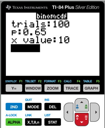
Fill in the parameters: trials = number of trials (n), p = binomial probability, x = number of successes (we've used $k$ on this page).

Just calculate. The reason for "paste" is that you're running a program to construct a command line. "Paste" pastes it to the command line where you can do the calculation by hitting [ENTER].
Example 3
Which is the appropriate distribution?
A candy manufacturer tells us that 15% of the candies manufactured and bagged in the factory are orange. Should we be surprised if a simple random sample of 25 candies contains 8 orange candies (i.e. 32% orange)?
$$\sigma_p = \sqrt{\frac{p(1-p)}{n}} = \sqrt{\frac{0.15(0.85)}{25}} = 0.0714$$
Now if we take this sample to be normal, that is, it follows a normal distribution $N(0.15, 0.0714)$, then we can calculate a Z-score for a proportion of 32%:
$$Z = \frac{0.32 - 0.15}{0.0714} = 2.38$$
Now the probability of this Z-score or lower (using the standard normal distribution) can be calculated on a TI-84 calculator like this:
normalcdf(2.38, 1E99, 0, 1) = 0.0087
So there's only a 0.9% chance of getting eight or more orange candies
But ...
If we take a closer look, this is really a binomial problem. First, it satisfies all four of the essential conditions for a binomial situation:
- There is a fixed probability of "success," getting an orange candy.
- We are consistently using the same sample size, $n = 25$.
- We have a binary outcome: A candy is either orange or it's not.
- Samples are independent. We assume that removing a small sample from a large pool will be independent of having taken other samples.
Further, these samples fail the large-cound conditions:
$$ \begin{align} np &= 25(0.15) = 3.75 \\[5pt] n(1-p) &= 25(0.85) = 21.25 \end{align}$$
We have $np \lt 10$, so we conclude that the normal approximation is not a good one in this situation. Just to put a cap on it, here's a picture of the appropriate binomial distribution for $n = 25$ and $p = 0.15$.
.png)
This distribution is smashed over to the left and has a long right tail; it's not normal. The binomial probability of finding eight orange candies in a pool of 25 is
$$ \begin{align} P(25, 8) &= \binom{25}{8} (0.15)^8 (1-0.15)^{17} \\[5pt] &= 1,081,575 \cdot (0.15)^8 (1-0.15)^{17} \\[5pt] &= 0.0175 \end{align}$$
So the binomial probability is 1.75%. It's a little higher than we found using the normal approximation. It would indeed be somewhat surprising to find eight orange candies in a random sample of 25, but not impossible.
Mean and variance of a binomial distribution
The mean of a binomial distribution is $\mu = np$.
The variance is $\sigma^2 = n p (1 - p)$
and the standard deviation is $\sigma = \sqrt{n p (1 - p)}$, where $p$ is the probability and n is the number of trials.
Example 4
An unbiased coin is tossed ten times. Calculate the probability of obtaining
- fewer than 4 heads;
- more than 7 heads.
- Calculate the mean and standard deviation of this distribution.
The probabilities are
$$ \begin{align} P(0) &= \binom{10}{0} \cdot 0.5^10 \cdot 0.5^0 \\[5pt] &= 1 \cdot (0.5^10) = 9.76 \times 10^{-4} \\[8pt] P(1) &= \binom{10}{1} \cdot 0.5^9 \cdot 0.5^1 \\[5pt] &= 10 \cdot 9.76 \times 10^{-4} = 9.76 \times 10^{-3} \\[8pt] P(2) &= \binom{10}{2} \cdot 0.5^8 \cdot 0.5^2 \\[5pt] &= 45 \cdot 9.76 \times 10^{-4} = 0.0439 \\[8pt] P(3) &= \binom{10}{3} \cdot 0.5^7 \cdot 0.5^3 \\[5pt] &= 120 \cdot 9.76 \times 10^{-4} = 0.117 \end{align}$$
So the total probability is the sum, $P(\lt 4) = 0.172$.
This could also be calculated by entering the function
binomcdf(10,0.5,3) = 0.1719
on a TI-84 calculator.
For part (b), we can just use the binomcdf() calculator function to calculate the probability of tossing 7 heads or fewer, and subtract that from 1.
binomcdf(10,0.5,7) = 0.9453
So the probability is $1 - 0.9453 = 0.0547$ or about 5.5%.
Finally (c), the mean of this distribution is $\mu = np = 10(0.5) = 5$, which means that, on average, 10 heads will result from every 10 tosses. The standard deviation is
$$\sigma = \sqrt{n p (1 - p)} = sqrt{10 \cdot 0.25} = 1.58$$. So the mean ± one standard devation is $\mu = 5 ± 1.6$.
Example 5
When a shipment of writing pens arrives at a wholesale warehouse, ten of them are tested. The entire shipment is returned if more than one of the sample is found to be faulty. Calculate the probability that the shipment will be accepted if 2% of the pens are faulty.
The probabilities are
$$ \begin{align} P(0) &= \binom{10}{0} \cdot 0.5^10 \cdot 0.5^0 \\[5pt] &= 1 \cdot (0.5^10) = 9.76 \times 10^{-4} \\[8pt] P(1) &= \binom{10}{1} \cdot 0.5^9 \cdot 0.5^1 \\[5pt] &= 10 \cdot 9.76 \times 10^{-4} = 9.76 \times 10^{-3} \\[8pt] P(2) &= \binom{10}{2} \cdot 0.5^8 \cdot 0.5^2 \\[5pt] &= 45 \cdot 9.76 \times 10^{-4} = 0.0439 \\[8pt] P(3) &= \binom{10}{3} \cdot 0.5^7 \cdot 0.5^3 \\[5pt] &= 120 \cdot 9.76 \times 10^{-4} = 0.117 \end{align}$$
So the total probability is the sum, $P(\lt 4) = 0.172$.
This could also be calculated by entering the function
binomcdf(10,0.5,3) = 0.1719
on a TI-84 calculator.
For part (b), we can just use the binomcdf() calculator function to calculate the probability of tossing 7 heads or fewer, and subtract that from 1.
binomcdf(10,0.5,7) = 0.9453
So the probability is $1 - 0.9453 = 0.0547$ or about 5.5%.
Finally (c), the mean of this distribution is $\mu = np = 10(0.5) = 5$, which means that, on average, 10 heads will result from every 10 tosses. The standard deviation is
$$\sigma = \sqrt{n p (1 - p)} = \sqrt{10 \cdot 0.25} = 1.58$$. So the mean ± one standard devation is $\mu = 5 ± 1.6$.
Practice problems — 2
-
Suppose we've discovered a "loaded" six-sided die. When tossed 1000 times in a test, it came up showing five 250 times.
- Calculate the expected value (mean) and standard deviation of a single roll of this die.
- Calculate the probability of rolling six 5's in 12 rolls of this die.
- Calculate the probability of rolling more than six 5's in 12 rolls.
Solution
First, we should calculate the probability of rolling a five with this die. From the information we have, that's
$$p = \frac{250}{1000} = 0.25$$
We ought to also check whether a binomial treatment is appropriate. We have (1) The outcome is binary – we either roll a 5 ("success") or we don't. (2) The number of trials (12) is fixed, (3) The probability of success is fixed $(p = 0.25)$ and (4) Each roll is independent.
For (a), the mean is $np = 12(0.25) = 3$. Three fives would be expected of this die in 12 rolls. The standard deviation is
$$ \begin{align} \sigma &= \sqrt{n p (1-p)} \\[5pt] &= \sqrt{12 \cdot 0.25 \cdot 0.75} \\[5pt] &= 1.5 \end{align}$$
So the mean is $\bar X = 3 ± 1.5$ rolls.
For (b), we want
$$ \begin{align} P &= \binom{12}{6} (0.25)^6 (0.75)^{12-6} \\[5pt] &= 924 (2.4414 \times 10^{-4})(0.1779) \\[5pt] &= 0.04 \end{align}$$
So there's a 4% chance of rolling six 5's in 12 rolls.
For (c), we can use the binomcdf() function on a TI-84 calculator:
binomcdf(12,0.25,6) = 0.9857
Now the calculator integrates (adds area under) the curve from left to right, so this is the probability of six or fewer successes. In order to find the probability of six or more successes, we have to calculate
binomcdf(12,0.25,5) = 0.9456
Then we subtract that probability from one:
$$1 - 0.9456 = 0.0544$$
So the probability of rolling six or more 5's in 12 rolls is 5.4%.
-
A certain car part is found to have an early failure rate of 12%. That is, 12 out of every 100 such parts will fail before its expected lifetime. A company wants to buy a fleet of 100 vehicles that contain this part.
- Calculate the probability that only one of the 100 fleet vehicles will contain the defective part.
- Calculate the probability that fewer than 5 of the fleet vehicles will contain the defective part.
Solution
Let's first check whether a binomial treatment is appropriate. We have (1) The outcome is binary – the part is either defective ("success") or it is not. (2) The number of trials (100) is fixed, (3) The probability of success is fixed $(p = 0.12)$ and (4) We assume that the selection of each vehicle is independent.
For (a), we're looking for the probability
$$ \begin{align} P &= \binom{100}{1} 0.12^1 (1-0.12)^{99}\\[5pt] &= 100 (0.12) (3.189 \times 10^{-6} \\[5pt] &= 0.004% \end{align}$$
Here, the probability of having a defective part is large enough to make the probability that just one vehicle out of 100 has one very small.
For (b) we want the probability that 5 or fewer vehicles will have the defective part. We'll use binomcdf() on the TI-84:
binomcdf(100,0.12,5) = 0.0152
So the probability that 5 or fewer vehicles will have the defective part is 1.5%. For comparison, let's run the same calculation asking for the probability that 20 or fewer vehicles will be affected:
binomcdf(100,0.12,20) = 0.9927
Now that probability is over 99%, so we need to be careful about our conclusions the first calculation came out with such a low probability because, given the relatively high incidence of defective parts, it was unlikely for such a small number of vehicles to be affected.
-
This problem is known as the drunkard's walk. A drunk is ten steps away from the edge of a pier. Every step he takes is either toward or away from the edge. He is equally likely to move in either of those directions each step he takes. Calculate the probability that he will fall into the water on his 10th step. How about his 20th step?
Solution
This is a binomial distribution problem, suitable for a cumulative probability distribution analysis [binomcdf()].
Here's the idea. We can calculate the probabilities of sums of steps. Forward steps are positive (+1) and backward steps are negative (-1). If the sum is greater than ten, then our drunk has fallen off the pier. If it's less, he's OK.
This is a binomial problem because (1) the steps are either forward ("success") or backward), (2) We choose a number of steps to examine (in the first problem it's 10, in the second it's 12, but those are separate questions, (3) the probability is the same for each step, $p = 0.5$, and (4) each step is independent of the others.
For the first question, we're asking for the probability that all ten of ten steps will be in the forward direction. That ought to be small. Let's see:
$$ \begin{align} P &= \binom{10}{10} (0.5)^{10} (1-0.5)^0 \\[5pt] &= 1 (9.765 \times 10^{-4}) (1) \\[5pt] &= 9.765 \times 10^{-4} \end{align}$$
So the probability is 0.0098%, very small as we'd suspected. It should be unlikely to take ten random steps all in the same direction. Now let's consider 20 steps.
$$ \begin{align} P &= \binom{20}{10} (0.5)^{10} (1-0.5)^{20-10} \\[5pt] &= 184,756 (9.765 \times 10^{-4}) (9.765 \times 1-^{-4}) \\[5pt] &= 9.765 \times 10^{-4} \end{align}$$
(under construction ... stand by)
dichotomy
A dichotomy is a situation in which only one of two constrasting things can be true. The phrase "It's either this or that" is a dichotomy.
In popular culture, especially political speech, we often encounter false dichotomies, in which only two choices are offered, but others exist.
normalized
A normalized probability distribution has been adjusted so that the total probability of any possible events happening is one.
A normalized vector has a length of 1.

![]()
xaktly.com by Dr. Jeff Cruzan is licensed under a Creative Commons Attribution-NonCommercial-ShareAlike 3.0 Unported License. © 2012-2019, Jeff Cruzan. All text and images on this website not specifically attributed to another source were created by me and I reserve all rights as to their use. Any opinions expressed on this website are entirely mine, and do not necessarily reflect the views of any of my employers. Please feel free to send any questions or comments to jeff.cruzan@verizon.net.