This section is an extension of the chemical kinetics page. Because calculus is the mathematics of change (like reaction rates), it's the best tool for finding reaction rate laws, or so-called integrated rate laws. If you don't know caclulus yet, it's OK to just accept the results gathered in the "integrated rate laws" box below.
Using calculus to integrate rate equations
Rates of all kinds should remind us of calculus, and indeed, calculus – differentiation and integration of functions – is an important part of analyzing the kinetics of a reaction. More specifically, chemical rate equations are (usually simple) differential equations, which we have the tools to solve.
In this section we'll work through a few examples of how to integrate rate laws to come up with useful equations that help us analyze what's going on kinetically in chemical processes.
Zeroth-order reaction
Consider a simple chemical process
![]()
that obeys a zero-order rate law (meaning that the exponent of [A] is zero:
$$Rate = k[A]^o$$
We can re-express the word "Rate" as the change in the concentration of A over time, or equivalently as the change in B over time. We'll choose the former and make sure that the rate is negative because we expect to be losing A:
$$\frac{- d[A]}{dt} = k$$
Now integrating this simple differential equation is easy
$$\int d[A] = \int k \, dt$$
The indefinite integral is
$$[A] = -kt + C$$
Now at time t = 0, we'll call the concentration of A "[A]o". Plugging in t = 0 and [A] = [A]o, we get
$$A_o = C$$
The integrated rate expression is
$$[A] = [A]_o - kt$$
The concentration of A plotted vs. time will yield a linear graph with intercept [A]o and slope -k.

So a zero-order reaction might be identified by plotting [A] vs. time and checking for a linear graph. If it is linear, then the slope of that graph will be the rate constant. An example of a zero-order reaction is the decomposition of ammonia:
First-order reaction
Sticking with our simple model equation, A → B, but now assuming that this is a first-order reaction, that is, it obeys the rate law
$$Rate = k[A]$$
we can substitute a derivative for "Rate."
$$\frac{-d[A]}{dt} = k[A]$$
This separable differential equation can be separated like this:
$$\frac{d[A]}{[A]} = k \, dt$$
Then we can integrate both sides. Notice that the integral on the left suggests a log function solution.
$$\int \frac{d[A]}{[A]} = -\int k \, dt$$
The integrated equation is
$$ln[A] = -kt + C$$
Now if we let [A]o be the concentration of A at time t = 0, we get the integrated equation for this first-order reaction:
$$ln[A] = -kt + ln[A]_o$$
This suggests that if we suspect that such a reaction is first order, and we plot ln[A] vs. time (t), we should obtain a linear graph with slope = -k and y-intercept ln[Ao].

Second-order reaction
Keeping with our simple model equation, A → B, but this assuming that this is a second-order reaction, that is, it obeys the rate law
$$Rate = k[A]^2$$
The differential equation is
$$\frac{-d[A]}{dt} = k[A]^2$$
It is separable, and the variable-separated form is
$$\frac{-d[A]}{[A]^2} = k \, dt$$
The integral is also a simple one
$$\int \frac{d[A]}{[A]^2} = \int k \, dt$$
The general solution is
$$\frac{1}{[A]} = kt + C$$
And once again if we let [A]o be the concentration of A at time t = 0, we get the integrated equation for this second-order reaction:
$$\frac{1}{[A]} = kt + \frac{1}{[A]_o}$$
This equation suggests that if we suspect a rate equation is second order in one component, a plot of 1/[A] vs. t should yield a linear graph with a slope of k and a y-intercept of 1/[A]o.

Example 1
Find the rate law and calculate the rate constant from the data.
C12H22O11 (aq) + H2O (l) → 2 C6H12O6 (aq)
The following concentration measurements were made at the time intervals shown, at 23˚C and in a weak HCl solution:
| Time (min.) | [C12H22O11] |
|---|---|
| 0 | 0.315 |
| 40 | 0.275 |
| 80 | 0.235 |
| 140 | 0.190 |
| 210 | 0.145 |
In a problem like this, we have concentration vs. time data. We don't know whether it's zero, first or second order kinetically – or perhaps even more complicated. We'll start by assuming that the rate law looks pretty much like this:
![]()
Now we can make good use of the fact that zero- first- and second-order data can be plotted in different ways, and the correct model should yield a linear graph. We'll begin by looking at the possibility that this is a zero-order reaction, and plotting [A] vs time:

This graph isn't too curved. In fact, the R2 value of a linear fit (blue line) yields a correlation coefficient of 0.995. Still, it's clear from the magenta line that there is a slight upward curvature. Maybe we can do better.
If this reaction is first order, a plot of 1/[A] vs. t should yield a linear graph:

Well, that's a little worse, with a clear upward curvature and a lower linear correlation, so we'll rule out first order.
How about second order? A plot of ln[A] vs time has the highest linear correlation and just by looking there is little if any curvature.

From this data set, we'd have to conclude that this is a second-order reaction. That means that the detailed mechanism likely depends upon some sort of collision and interaction between two sucrose molecules before they break apart into fructose and glucose.
One thing you've probably noticed is that the distinction of reaction orders was pretty subtle here. It's often more obvious, but kinetic measurements and data can be tricky. That's the way it is. It often takes a great deal of data of various types to fully understand the kinetic details of a reaction.
The rate constant, k, is the slope of our line, so k = 3.6 × 10⁻³, and the units of rate must be molarity/second, so the units of k are M-1·s-1
Example 2
Determine the order of the reaction 2N2O5 (g) → 4NO2 (g) + O2 (g) from the data.
| [N2O5] (M) | Time (s) |
|---|---|
| 0.100 | 0 |
| 0.709 | 50 |
| 0.051 | 100 |
| 0.249 | 200 |
| 0.126 | 300 |
| 0.0063 | 400 |
We'll follow the same procedure as above, plotting graphs to determine whether this is a zero-, first- or second-order reaction.
Zero order
From this data we can clearly see that the plot of [N2O5] vs. time is non-linear, so we can rule the zero-order case out.

First order
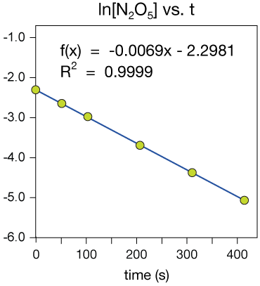
The plot of ln[N2O5] vs time is linear, with a correlation coefficient very near 1. This looks like first-order kinetic data.
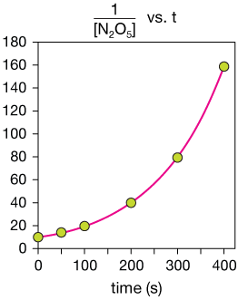
Second-order
The plot of the reciprocal of [N2O5] vs time is also clearly non-linear, so now we can be sure that this is a first order reaction.
The reaction is first order and the rate constant comes from the slope of the ln[N2O5] vs. time graph, k = 0.0069 s-1 (different units than the last example!)
Integrated rate laws

The half life
Very often when measuring data on the rate of a reaction, it is more convenient to measure the time it takes for the concentration of a reactant to be reduced to one-half it's starting concentration — and then to ¼ ⅛ and so on. The time that it takes for such a concentration reduction is called the half life.
The half life is widely used in nuclear chemistry, too. In this section we'll use our integrated rate laws to find the half-life formulas of zero, first and second-order reactions, and see how they can help to understand kinetic data.
Zeroth-order half life
the zeroth-order rate law is
$$[A] = [A]_o - kt$$
The trick to finding the half-life expression is, first, to solve for time, t, and then to replace [A] with [A]o/2. First solve for t:
$$\frac{[A] - [A]_o}{-k} = t$$
Then substitute [A]o/2 for [A] and simplify to get the half life formula:
$$t_{1/2} = \frac{[A]_o}{2k}$$
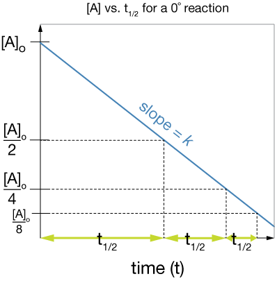
Notice that the half-life for a zero-order reaction is dependent on the initial concentration.
Here is a plot of [A] vs. t for such a reaction with some half-lives sketched in so you can see the concentration dependence:
First-order half life
We follow the same procedure as above for determining the half-life for a first-order reaction. Fist, the integrated rate law (one version of it) is:
$$ln[A] = -kt + ln[A]_o$$
Isolating the time gives
$$\frac{ln[A] - ln[A]_o}{-k} = t$$
Now we'll use the property of logs that ln(x) - ln(y) = ln(x/y) to rearrange:
$$\frac{1}{-k} \cdot \frac{ln[A]}{ln[A]_o} = t$$
Now substitute t1/2 for t, and at that time, [A] = [A]o/2:
$$\frac{1}{-k} \cdot \frac{ln([A]_o/2}{ln[A]_o} = t$$
Dividing the [A]o gives a simple log of a constant in the numerator, which we can approximate:
$$\frac{ln\left( \frac{1}{2} \right)}{-k} \approx \frac{0.693}{k} = t_{1/2}$$
Now here's what's strikingly different between the half life of a first order reaction and that of a zero-order reaction: It doesn't depend at all on the initial concentration [A]o
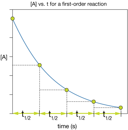
The specific shape of the [A] vs. t curve for a first-order reaction ensures that each half-life is the same. This is a unique feature of a first-order reaction like this.
Second-order half life
Finally, let's find an expression for the half life of a second-order reaction. We begin again with the integrated rate law:
$$\frac{1}{[A]} = kt + \frac{1}{[A]_o}$$
Isolating the kt term gives
$$kt = \frac{1}{[A]} - \frac{1}{[A]_o}$$
This is a convenient step to convert to half life:
$$kt_{1/2} = \frac{1}{[A]_o/2} - \frac{1}{[A]_o}$$
Rearranging the first fraction gives a nice expression for kt1/2:
$$kt_{1/2} = \frac{2}{[A]_o} - \frac{1}{[A]_o} = \frac{1}{[A]_o}$$
And dividing by k gives us our result:
$$t_{1/2} = \frac{1}{k [A]_o}$$
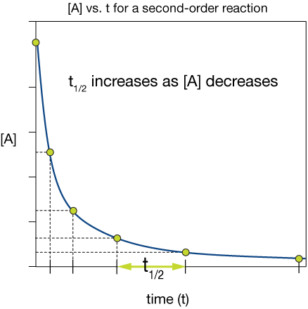
So the second-order half life depends on the reciprocal of the initial concentration of the second-order reactant.
The plot of [A] vs t for a second-order reaction below shows that as the initial concentration decreases, the half life increases, as we'd expect from the half-life expression.

![]()
xaktly.com by Dr. Jeff Cruzan is licensed under a Creative Commons Attribution-NonCommercial-ShareAlike 3.0 Unported License. © 2012, Jeff Cruzan. All text and images on this website not specifically attributed to another source were created by me and I reserve all rights as to their use. Any opinions expressed on this website are entirely mine, and do not necessarily reflect the views of any of my employers. Please feel free to send any questions or comments to jeff.cruzan@verizon.net.