A very handy use of the derivative
Now that you've learned how to find the derivative of most functions, this section and the next (curve sketching) will show you some key applications. The first is making linear approximations of nonlinear functions.
Making linear approximations (and later quadratic approximations) can be very handy for finding high-quality approximations of difficult or complicated functions.
Often, we can vastly simplify a problem without loss of real accuracy by making a linear approximation using calculus.
Later we'll learn to improve our approximations, in some cases to as much precision as we'd like. Converting a function like $f(x) = \text{sin}(x)$ to a polynomial approximation (yes, you will learn to do that) for example, can be invaluable for doing more complicated mathematical modeling.
Linear approximations
When viewed at a sufficiently fine scale, any curve resembles a line. In the graph below, the function $y = L(x)$ is not a bad approximation of $y = f(x)$ in the "neighborhood" around $x_o$.

If $L(x)$ is the derivative of $f(x)$ at $x_o$, then, recalling that the equation of a line can be found using the point-slope formula,
$$y - y_o = m(x - x_o)$$
we find
$$L(x) - f(x_o) = f'(x_o)(x - x_o)$$
If we agree that our function $f(x)$ is approximately equal to $L(x)$ near $x_o$, then we have:

which is the equation of a tangent line passing through the point $(x_o, \; f(x_o))$. We presume that the approximation is better the closer $x$ is to $x_o$. Depending on the shape of $f(x)$, our approximation can be terrific over quite a range of $x$, or not so good. We'll have to figure out how to evaluate that later.
Linear approximation of f(x)
When viewed at a fine-enough scale, any curve is approximately a line. We can approximate curves using the derivative.
The linear approximation of a function near a point on its graph is simply the equation of the line tangent to the function at that point:
$$f(x) \approx f'(x_o)(x - x_o) + f(x_o)$$
Example 1
Find a linear approximation of $f(x) = ln(x)$ near $x = 1$.
From the equation in the green box, we see that we need the value of $f(x_o)$,
$$f(1) = 0$$
and the value of the derivative at $x_o$, $f'(x_o)$,
$$f'(x) = \frac{1}{x} \: so \: f'(1) = 1$$
Putting it all together, we have
$$ \begin{align} f(x) &\approx f(x_o) + f'(x_o)(x - x_o) \\[5pt] &= 0 + 1\cdot(x - 1) = x - 1 \\[5pt] &= x - 1 \end{align}$$
So the contention is that in the neighborhood of $x_o=1$, the function $f(x) = ln(x)$ is approximately equal to $x - 1$.
Here's a graph that will illustrate the point:

As long as we stay near $x = 1$, this approximation is "pretty good." It gets worse as we move away from 1 in either direction along the x-axis, and we'll define "worse", and "good" and "bad" approximations as we go along.
When making approximations, it's always important to evaluate the quality of an approximation. I could approximate my weight at 1 lb., but it wouldn't be a good approximation.
Approximations around $x = 0$
It's handy to make our approximations around $x = 0$ instead of $x = 1$. That is, we'll set and the value of $x_o=0$. We'll see why a little later, but for now, let's see what affect that has. We'll start out with the definition of the linear approximation from above:
$$f(x) - f(x_o) \approx f'(x_o)(x - x_o)$$
If we insert $x_o=0$, it's considerably simpler:
$$f(x) \approx f(0) + f'(0) x$$
Now let's calculate linear approximations of the functions $f(x) = \text{sin}(x)$, $f(x) = \text{cos}(x)$ and $f(x) = e^x$ because we use those a lot.
We'll need values of $f(0)$, $f'(x)$ and $f'(0)$, so let's make a handy table and calculate them, then we'll add the terms to get our approximations.
| $f(x)$ | $f(0)$ | $f'(x)$ | $f'(0)$ | $f(0)+f'(0)x$ |
|---|---|---|---|---|
| $\text{sin}(x)$ | $0$ | $\text{cos}(x)$ | $1$ | $x$ |
| $\text{cos}(x)$ | $1$ | $-\text{sin}(x)$ | $0$ | $1$ |
| $e^x$ | $1$ | $e^x$ | $1$ | $1+x$ |
Our linear approximations are:
$$ \begin{align} \text{sin}(x) &\approx x \\[5pt] \text{cos}(x) &\approx 1 \\[5pt] e^x &\approx x + 1 \end{align}$$
Below are graphs of each of these three example functions (black) and their approximations near $x = 0$ (magenta). Notice that (1) very close to $x = 0$, these approximations are very good and (2) some are better than others. In particular, the linear approximation $\text{sin}(x) \approx x$ is very good because the sine function is more-approximately linear over a wider range in that region.
While the approximation of the cosine function is great just near $x = 0$, the curve is so tight there that it doesn't seem like the approximation will be very good even very near $x = 0$ ... but that's not very quantitative.


Example 2
Find a linear approximation of $f(x) = ln(1 + x)$ near $x = 0$
$$f(0) = ln(1) = 0$$
$$f'(x) = \frac{1}{1 + x}, \: \: and \: f'(0) = 1$$
which gives us
$$ln(1 + x) \approx x$$
Now let's see why this might be useful. Suppose we want to know the value of $ln(1.1)$
Now $ln(1.1) = ln(1 + 0.1)$. That means $x = 0.1$ in our approximation equation, so $ln(1.1) \approx 0.1$.
If I punch in $ln(1.1)$ on my calculator, I get $ln(1.1) = 0.0953101798$ ... not too shabby.
Let's calculate some other logs a little closer to and a little farther away from zero (that means x a little smaller/larger than zero) and see how we do:
| $f(x)$ | $x$ | approx. | calculator | $\Delta$ |
|---|---|---|---|---|
| $ln(1.05)$ | $0.05$ | $0.05$ | $0.0487901$ | $2%$ |
| $ln(1.1)$ | $0.1$ | $0.1$ | $0.0953101$ | $5%$ |
| $ln(1.2)$ | $0.2$ | $0.2$ | $0.1823215$ | $10%$ |
| $ln(1.5)$ | $0.5$ | $0.5$ | $0.4054651$ | $23%$ |
| $ln(2.0)$ | $1.0$ | $1.0$ | $0.6931472$ | $44%$ |
Clearly we get into trouble when we stray too far from x = 0. A 10% error for ln(1.2) might be too much to tolerate in some applications, and a 44% error in ln(2) certainly would be. On the other hand, we got within 2% of ln(1.05).
Example 3
Find a linear approximation of $f(x) = \sqrt{x + 1} \cdot e^{x + 1}$ near $x = 0$.
$$f(0) = e \: \: and \: \: f'(0) = \frac{3e}{2}$$
Plugging these into our expression for the linear approximation, we get
$$f(x) \approx e \left( 1 + \frac{3}{2}x \right)$$
Now let's again calculate some values of $f(x)$ both by our approximation and by the calculator, and examine the errors:

We see again that our simple linear approximation of this rather complicated function is pretty good when working with numbers from its domain very close to zero.
Why not just calculate f(x) directly?

A fair question. Why do all this approximating when a calculator or computer will do the work to high precision in just a few minutes?
One problem with functions like the one in the example above is that they take a relatively long time for a computer to compute. They involve a lot of multiplication (roots and exponentiation are performed with several multiplication steps
in a computer), the most time-consuming operation. Now if you've got to perform the same computation millions or billions of times, that can really add up. It may come down to this question: Do I do the calculation using the approximation and accept some small error, or do I go for high precision and never get it done?
Example 4
Use a linear approximation to calculate the value of (5.109)2, and compare it to the calculated value of 26.101881
We begin with the linear approximation form:
$$f(x) \approx f(x_o) + f'(x_o)(x - x_o)$$
and insert the values we're looking for, using $x_o=5$ and $x = 5.109$:
$$f(5.109) \approx f(5) + f'(5)(x - 5)$$
Now $f(5) = 25$, and we can plug everything in to get:
$$ \begin{align} &= 25 + (2.5)(5.109 - 5) \\[5pt] &= 26.109 \end{align}$$
We now have a simple formula for calculating squares of awkward numbers near 5. It's
$$x^2 = 25 + 10(x - 5)$$
which is actually pretty easy to do without a calculator.
Now the difference between our approximation and the calculated result is 0.007, or less than 0.1% from the actual value, which is probably pretty good for most applications.
A practical example – the pendulum

The equation of motion for a pendulum looks like this:
$$\frac{d^2\theta}{dt^2} = \frac{-g}{L} sin(\theta)$$
where $g$ is the acceleration of gravity ($g = 9.81 m/s^2$), $L$ is the length of the pendulum string and $\theta$ is the angle of the pendulum string from the vertical.
This second-order differential equation is difficult to solve because of the $\text{sin}(\theta)$ on the right. But as we learned in our examples above, for small angles, and to a very good approximation,
$$\text{sin}(\theta) \approx \theta$$
Plugging this approximation into our pendulum equation of motion gives
$$\frac{d^2 \theta}{dt^2} = \frac{-g\cdot\theta}{L}$$
Now this equation is much easier to solve (I'll omit the solution here as it's more advanced and not relevant to this section), and at small angles it's quite accurate.
Practice problems
-
Find a linear approximation of the square-root function near $x = 5$, and use it to approximate $\sqrt{5.525}.$
Solution
First find the specific point and slope. The point is
$$f(x) = \sqrt{x} \: \color{#E90F89}{\rightarrow} \: f(5) = \sqrt{5}$$
so our point is $(5, \, \sqrt{5}).$ The slope is
$$f'(x) = \frac{1}{2 \sqrt{x}} \: \color{#E90F89}{\rightarrow} \: f'(5) = \frac{1}{2 \sqrt{5}}$$
Now find the equation of the line:
$$ \begin{align} y - y_o &= m(x - x_o) \\[5pt] y - \sqrt{5} &= \frac{1}{2 \sqrt{5}} (x - 5) \\[5pt] y &= \frac{x}{2 \sqrt{5}} - \frac{5}{2 \sqrt{5}} + \sqrt{5} \\[5pt] y &= \frac{x}{2 \sqrt{5}} + \frac{\sqrt{5}}{2} \\[5pt] y &= \frac{x}{4.4721} + 1.11803 \end{align}$$
That is our linear approximation of our original function in the neighborhood of x = 5. Now our square root:
$$ \begin{align} \sqrt{5.525} &\approx \frac{5.525}{4.4721} + 1.11803 \\[5pt] &= 2.353 \end{align}$$
The calculator value is 2.351, for an error of about 0.1%, not too bad. If you needed to calculate a billion square roots of numbers near 5, this could save a considerable amount of computer time. You'd only actually calculate rots for the setup of the linear approximation.
-
Use a linear approximation to estimate tan(0.25). Compare your result to y = tan(0.25) from a calculator (use radians!).
Solution
We'll use an approximation centered at x=0 because that's our most convenient point close to x = 0.25.
$$ \begin{align} f(x) &= \text{tan}(x) \\[5pt] f(0) &= \text{tan}(0) = 0 \end{align}$$
So our point is (0, 0). Now the slope is obtained by calculating the derivative of f(x) at x = 0:
$$ \begin{align} f'(x) &= \text{sec}^2(x) \\[5pt] f'(0) &= \frac{1}{\text{cos}^2 (0)} = 1 \end{align}$$
The equation of the tangent line is
$$ \begin{align} y - y_o &= m (x - x_o) \\[5pt] y - 0 &= 1 (x - 0) \\[5pt] y = x \end{align}$$
That's a very simple linear approximation. It means that $tan(0.25) \approx 0.25.$ The calculated value is $tan(0.25) = 0.25534,$ which gives about a 2% error. Not too bad for the savings in computing speed. If you can tolerate this kind of error in your calculations – and that's situation dependent then this would be a good approximation in this region.
-
Use a linear approximation to estimate the value of 1/1003.
Solution
We'll center our approximation on x = 1000, a conveniently-round number near the x-value of interest. Our point on the function f(x) is
$$ \begin{align} f(x) &= \frac{1}{x} \\[5pt] f(1000) &= \frac{1}{1000}, \: \text{so} \\[5pt] (x, y) &= \left( 1000, \, \frac{1}{1000} \right) \end{align}$$
The slope at x = 1000 is:
$$ \begin{align} f'(x) &= \frac{-1}{x^2} \\[5pt] f'(1000) &= \frac{-1}{1000^2} \end{align}$$
Now our linear approximation formula is
$$ \begin{align} y - y_o &= m (x - x_o) \\[5pt] y - \frac{1}{1000} &= \frac{-1}{1000^2} (x - 1000) \\[5pt] y &= \frac{-x}{1000^2} + \frac{1}{1000} + \frac{1}{1000} \\[5pt] y &\approx \frac{-x}{1000^2} + \frac{2}{1000} \end{align}$$
The approximate value of 1/1003 is then
$$ \begin{align} \frac{1}{1003} &\approx \frac{2000 - 1003}{10^6} \\[5pt] &= 997 \times 1-^-6 \\[5pt] &= 0.000997 \end{align}$$
That approximation is exact to the precision shown above.
-
Use a linear approximation of f(x) = 2x3 - 6x2 to approximate f(2.4).
Solution
Point:
$$ \begin{align} f(x) &= 2x^3 + 6x^2 \\[5pt] f(2) &= 2(8) + 6(4) = 40 \end{align}$$
Slope:
$$ \begin{align} f'(x) &= 6x^2 + 12x \\[5pt] f'(2) &= 24 + 24 = 48 \end{align}$$
The equation of our linear approximation to the function is
$$ \begin{align} y - y_o &= m(x - x_o) \\[5pt] y - 40 &= 48(x - 2) \\[5pt] y &= 48x - 56 \end{align}$$
Now we can calculate our approximation of f(2.4):
$$ \begin{align} f(2.4) &\approx 48(2.4) - 56 \\[5pt] &= 115.2 - 56 \\[5pt] &= 59.2 \end{align}$$
The exact value (to the thousandths place) is 62.208, a 4.8% error. Every linear approximation of a function is different, and depends on the amount of curvature present in the function at the point of interest.
-
Use a linear approximation to estimate e-1.015.
Solution
Point:
$$ \begin{align} f(x) &= e^x \\[5pt] f(-1) &= \frac{1}{e} \\[5pt] (x, y) &= \left( -1, \, \frac{1}{e} \right) \end{align}$$
Slope:
$$ \begin{align} f'(x) &= e^x \\[5pt] f'(-1) &= \frac{1}{e} \end{align}$$
The equation of our linear approximation to the function is
$$ \begin{align} y - y_o &= m(x - x_o) \\[5pt] y - \frac{1}{e} &= \frac{1}{e}(x + 1) \\[5pt] y &= \frac{x}{e} + \frac{2}{e} = \frac{x + 2}{e} \end{align}$$
Now we can calculate our approximation of f(-1.015):
$$ \begin{align} f(-1.015) &\approx \frac{2 - 1.015}{e} \\[5pt] &= 0.3624 \end{align}$$
To the precision given, this solution, $e^{-1.015} = 0.3624,$ is exact.
Quadratic approximations
We'll close out this section by introducing, without any sort of derivation, a formula for adding a quadratic term to such an approximation. This is an effort to improve on our linear approximations. We'll apply it to three functions, $f(x) = \text{sin}(x)$, $f(x) = \text{cos}(x)$ and $f(x) = e^x$, so that we can compare the results to the linear approximations we derived above.
The second term includes the second derivative - the derivative of the derivative, which we can label $f'(x)$. The formula is:
$$f(x) \approx f(0) + f'(0)x + \frac{f''(0)}{2} x^2$$
I won't bother to elaborate on the origin of this new term; that will come later when we learn about series. For now, let's rebuild our table of values of $f(0)$ and $f'(0)$, and add $f''(0)$ to get our quadratic approximations.
The table below shows that the approximation for the sine function doesn't change upon addition of this new term — its value is zero. That makes some sense because in the derivation of the linear approximation above, the line $y = x$ seemed like a pretty darn good approximation for $\text{sin}(x)$ around zero.
The approximation of $\text{cos}(x)$ is improved by addition of the term $-x^2/2$, a downward-opening parabola. The graph below (left) shows that new approximation superimposed upon $y = \text{cos}(x)$. Clearly this approximation would be better over a wider range of the domain near $x = 0$.
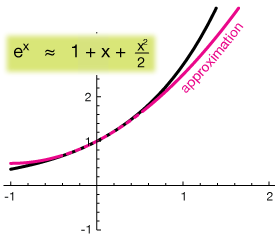
Finally, the approximation of $e^x$ is also improved by addition of an upward-opening parabola. The improvement adds some curvature to our linear approximation that is concave-upward, just like the function.

Here are graphs of the cosine and exponential functions showing how the new quadratic terms in our approximations bend them in the right direction to match the curvature of the function.


![]()
xaktly.com by Dr. Jeff Cruzan is licensed under a Creative Commons Attribution-NonCommercial-ShareAlike 3.0 Unported License. © 2012-2025, Jeff Cruzan. All text and images on this website not specifically attributed to another source were created by me and I reserve all rights as to their use. Any opinions expressed on this website are entirely mine, and do not necessarily reflect the views of any of my employers. Please feel free to send any questions or comments to jeff.cruzan@verizon.net.